
Setting the stage
The following piece of imperative-style pseudo code (taken from [1]) is one way¹ to implement John Conway’s celebrated “Game of Life”. Before inspecting the code, you may want to quickly find out what the “Game of Life” (GoL) actually is, e.g. here: https://academo.org/demos/conways-game-of-life/.
def life_evaluation( cells ):  # cells is a 3x3 array
 count = 0
 for i in [0,1,2]:
   for j in [0,1,2]:
     if i!=1 and j!=1:
       count += cells[i,j]
 return life_count_evaluation( cells[1,1],count )

def life_count_evaluation( cell,count ):
 if count<2:
   return 0    # loneliness
 elif count>3:
   return 0    # overcrowding
 elif cell==1 and (count==2 or count==3):
   return 1    # live on
 elif cell==0 and count==3:
   return 1    # spontaneous generation
 else:
   return 0    # no change in dead cells

def life_generation( board,tmp ):
 for i in [0:N-1]:
   for j in [0:N-1]:
     tmp[i,j] = board[i,j]
 for i in [0:N-1]:
   for j in [0:N-1]:
     board[i,j] = life_evaluation( tmp[i-1:i+1,j-1:j+1] )

# create an initial board; we omit this code
life_board.create(N,N)
temp_board.create(N,N)

# now iterate a number of steps on the whole board
for t in [0:final_time-1]:
  life_generation( life_board,temp_board )
Having absorbed the preceding barrage of information, you may have come to sense that “Life is just one damn thing after another”². Well, that impression would be right. Of course, only insofar as we are talking about the implementation (which takes nothing away from the “alluring, transfixing, infectious complexity” which can arise from the Game of Life’s elegantly minimalistic laws [2]). In [1] it is referred to as the basic “sequential implementation, since it does its computation in a long sequence of steps.” (See Figure 1 for an example of three time-steps in the Game of Life.) Each time-step is computed one after the other (as you can tell from the final “for loop”), as is also each cell within each time-step.
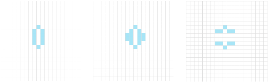
Figure 1: An example of a sequence of three time-steps in the Game of Life. Source: https://academo.org/demos/conways-game-of-life/
But this is not a logical requirement of the problem. Each cell’s state at t+1 can be computed in parallel (as a cell’s state at t+1 does not depend on any other cell’s state at t+1, only on its neighbours’ state at t). Even computing the time-steps in strict sequence is not a necessity. As an example, a patch of 5x5 cells at time t would be sufficient to compute the cell i,j at t+2 (you might be able to intuit that the state of a cell can be computed for two time-steps by considering a range of neighbouring cells at most two cells apart in the i or j direction). So as far as this cell is concerned, there is no need to wait for t+1 in some other part of the board to be computed first.
Opportunities therefore abound for escaping the tedium of computing GoL sequentially. But what are the means to eliminate sequential execution, in particular where it is “an artefact of the programming language”, as opposed to a logical requirement of the problem [1]?
In [1], the reader is guided through some available techniques and includes a number of segues into relevant hardware considerations. For instance, in discussing the idea that multiple cells may be updated in parallel via so-called “vector instructions”, as these are well “matched to the innermost components of a processor core “ (at a stretch, we may imagine this facility being applied to the computation of the “count” variable – which tracks the number of neighbouring cells which are alive – in the inner loop of “life_evaluation”).
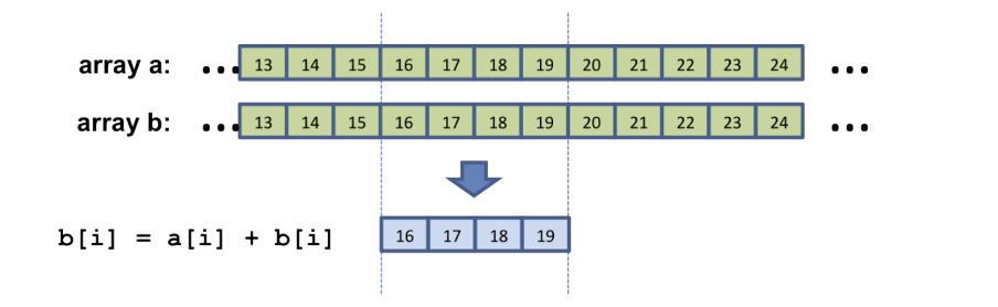
Figure 2: Instead of operating on a single pair of inputs, you would load two or more pairs of operands, and execute multiple identical operations simultaneously. Applied to our case, instead of the variable “count” being associated with a single cell, we treat it as an array, whereby the elements of this array are in relation to an array of cells on the board. The idea is to update multiple elements of this array simultaneously. Source: [1]
Figure 2 illustrates the idea of vector instructions. If, however, this still leaves you feeling unsure as to how exactly you would summon this power of parallelism (hint: [1] mentions the “loop unrolling” technique), rest assured that – in the imperative programming paradigm – adding “parallelism is not a magic ingredient that you can easily add to existing code, it needs to be [an] integral part of the design of your program” [1]. Like the character Glendower in Shakespeare’s King Henry IV, you can call the spirits from the vasty deep. But having to rely (to some extent) on the compiler’s ability to figure out when vector instructions can be used [1] is reminiscent of Hotspur’s taunting counter:
Why, so can I, or so can any man;
But will they come when you do call for them?
Interlude
So far I have alluded to a form of so-called data parallelism. The same instruction being performed on multiple data elements (i.e., a bunch of cells within a given row or column) at the same time. But what if, in addition, we wanted different regions of the board to be processed in parallel? Before addressing that, let us take a step back from Life.
If our grand goal is to eliminate artificial “sequentialism”, ideally it would be our aim to let data dependencies “locate parallelism” [3]. This is, perhaps, an odd way of saying that we want parallel execution to be the norm, except where data dependencies require a logical order to the computation. Clearly, this is idealistically put, as it assumes that any number of instructions can be executed in parallel – in reality, we are limited to a finite number of processing elements (it also implies unbounded buffering capacities, which is unrealistic) [3].
Entrance of the dataflow approach
Well, the spirit of this approach can be (partially) captured by following our guide [1] in an effort to distribute the program across multiple processors (or nodes), and employing a Message Passing Interface (MPI) library, which “adds functionality to an otherwise normal C or Fortran program for exchanging data with other processors”. We can make use of this approach to parallelize the computation of different regions of the board.
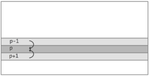
Figure 3: Processor p receives a line of data from p − 1 and p + 1. Source: [1]
As alluded to by Figure 3, we may split the board into a number of concurrent independent processes. Each can start chugging away, computing its line before any other line has been finished processing. To complete the work on each iteration, however, it does require that each process has received the current states of the adjacent lines on the board (this represents the data dependency).
The aforementioned approach is termed dataflow in [1]. Indeed, although it is also defined there, general use of the term doesn’t identify a very precise thing. The term can be a reference to the pure computational model, to hardware architectures, to one of a number of different dataflow language implementations, or, as in the preceding example, to a kind of technique that abstracts away from the underlying language implementation. In what follows, and possibly in a way that gives hand-waving a good name, I will try to pick out a few of the core properties, which (I would guess) are shared by most designs that lay claim to the dataflow label. The MPI example from above may represent somewhat of a special case, which does not live up to the billing entirely (although I lack the ambition to state precisely in what ways).
First is the “implicit achievement of concurrency [4].” That is, dataflow reduces the need for the programmer to explicitly “handle concurrency issues such as semaphores or manually spawning and managing threads [4].” This is made possible by the fact that dataflow consists of a number of independently acting “processing blocks”, which are each driven by the presence of input data (as opposed to an instruction, which, while input data may be available, must wait its turn in the program until the program counter reaches it). As a result, we are liberated from the sequential ordering imposed by a classical language’s execution model.
Take Figure 4 as an example. On the left we have a simple imperative program, on the right its dataflow equivalent. Whereas the assignment operation for B must wait in the imperative program until the first operation has completed, the first two operations may proceed concurrently in the dataflow program. We might call this kind of parallelism “task” parallelism, which would be the analogue of the MPI example discussed above. Note also, that while the operation for C is in progress, a second wave of computations may already be executing for the first two operations. This is known as pipeline parallelism and comes about naturally in the dataflow execution model. The equivalent of data parallelism, which was mentioned above, would be multiple instances of the same graph (or subgraph), with the input data streams partitioned such that each data item is fed into one or another of the running instances.
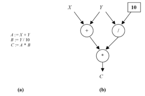
Figure 4: A simple program (a) and its dataflow equivalent (b). Source: [3]
Going a bit deeper, the dataflow diagram in Figure 4 can be understood as follows [3]:
“In the dataflow execution model, a program is represented by a directed graph. The nodes of the graph [in the pure dataflow model] are primitive instructions such as arithmetic or comparison operations. Directed arcs between the nodes represent the data dependencies between the instructions. Conceptually, data flows as tokens along the arcs which behave like unbounded first-in, first-out (FIFO) queues.”
Most expositions of the dataflow model point out this unifying connection between a dataflow program and a directed graph. Rarely, though, is an underlying explanation of this connection made explicit – perhaps, because it is too obvious. However, this visual property paves the way to visual programming, a very compelling advantage of the dataflow paradigm. It therefore seems a worthy property to ponder .
As the name suggests, a directed graph brings with it a sense of directionality. In Figure 4, the flow of data is visually guided by arrows. This representation is compatible with the dataflow model, since, in effect, the model imposes a unique relation between a dataflow variable and an arc. More technically, within each computational “wave”, dataflow variables are single-assignment variables (i.e., non-mutable). In a traditional, imperative-style programming language, this sense of directionality is not so evident. Here, variables may be thought of as containers in which a value may be stored and updated multiple times [5]. Take a statement, such as the following, which implies repeated variable assignment:
n = n + 1
Trying to model such a statement as a simple graph would imply that n is both an input arc to the addition operation (along with the input arc feeding the constant value of 1), as well as its output arc. This throws into chaos any attempt to build a graph representation. Hence, the notion of single-assignment variables looks to be rather important, and indeed, is seen as one of the distinguishing properties of the dataflow model. See in [5] for example, how this and other concepts are used to construct a taxonomy of programming paradigms!
A related property which makes the dataflow model amenable to the graph view is that it enforces pure data interfaces between the nodes. In other words, the graph’s set of arcs represent the entirety of the information transfer that happens between nodes – no other forms of informational “coupling” between modules are allowed (i.e. any form of control communication [6], such as data which might be interpreted as a flag used to control certain aspects of the execution of another module). The level of coupling in dataflow is in fact the minimal requirement for a functioning system [6]. In other words, “coupling is…minimized when only input data and output data flow across the interface between two modules” [6]. This approach to programming may seem restrictive, but in light of the reduction of complexity, it is in fact suggested as a general programming methodology by the authors of [6]³. “The great advantage of the dataflow approach is that “modules” interact in a very simple way, through the pipelines connecting them” [7].
Lastly, it is also instructive to notice what the graph view is devoid of, namely any expression controlling the dynamic behaviour of the program. In Figure 4, the order of the statements on the left is an expression of the order of execution. That is, the mere ordering of statements is expressing a flow of control. More generally, one can imagine the execution of a traditional program as jumping around the code of the program, whereby one single instruction is executed at a time.
By contrast, the graph on the right in Figure 4 does not convey whether the addition or the division operation should proceed first. It would therefore be inadequate to represent the operational semantics of an imperative program. Not so for the dataflow model. The programmer does not have to specify the dynamic execution behaviour, which is precisely one of dataflow’s advantages. Provided the input arcs have data on them (at which point the node/instruction is said to be “fireable”), the first two operations in Figure 4 may proceed concurrently. More generally, “if several instructions become fireable at the same time, they can be executed in parallel. This simple principle provides the potential for massive parallel execution [3]“. As more of an aside, this behaviour of waiting for available input data is expressed as, technically, waiting for a variable to be bound. The fact that [8] identifies dataflow with this very property – “this civilized behaviour is known as dataflow” – suggests its significance.
So that concludes some basic insights into dataflow. Clearly, much more can be said about this topic which has seen several decades of development. Indeed, the first clear statement of pipeline dataflow dates back as far as 1963 [7] – incidentally, made by a certain Conway (Melvin Conway in this case). Anyway, I hope that this blog has left you with an appetite for more.
References
|
V. Eijkhout, “Chapter 10 – Parallel programming illustrated through Conway’s Game of Life,” in Topics in Parallel and Distributed Computing, Boston, Morgan Kaufmann, 2015, pp. 299-321. |
|
|
S. Roberts, Genius at Play: The Curious Mind of John Horton Conway, London: Bloomsbury, 2015. |
|
|
Wesley, A. Johnston .J. R. Paul Hanna, and Richard J. Miller, “Advances in Dataflow Programming Languages,” ACM Computing Surveys, vol. 36, pp. 1-34, 2004. |
|
|
T. B. Sousa, “Dataflow Programming Concept, Languages, and Applications,” Doctoral Symposium on Informatics Engineering, vol. 130, 2012. |
|
|
P. Van Roy, Programming Paradigms for Dummies: What Every Programmer Should Know, 2012. |
|
|
Yourdon, Edward and Constantine, Larry L.; Structured Design: Fundamentals of a Discipline of Computer Program and Systems Design, USA: Prentice-Hall, Inc., 1979. |
|
|
Wadge, William W. and Ashcroft, Edward A.; LUCID, the Dataflow Programming Language, USA: Academic Press Professional, Inc., 1985. |
|
|
P. van Roy, H. Seif; Concepts, Techniques, and Models of Computer Programming, MIT Press, 2003. |
¹ Assuming we have a board of N×N cells and we would like to compute a certain number of timesteps. We also don’t care much for the edge of the board.
² This quote has been attributed to various people, among them Mark Twain.
³ Their method involves two separate stages; in the first (“program analysis”) the analyst produces a (pipeline) dataflow net that performs the necessary computations; then in the second stage (“program design”) the net is translated into the language at hand, usually COBOL [6].

